Manual Clustering Practical User's Guide
Note: This user's guide has been written by Stephen Lenzi (Margrie Lab) and Nick Steinmetz for an earlier version of phy. Please open issues or pull requests if updates to this page are needed for phy 2.0.
Contents:
- Some basic concepts
- Installation and requirements
- Running the GUI
- What is shown in the GUI
- Keyboard commands
- A practical guide to a typical approach to manual clustering
- What next? Getting started with analysis
- FAQ
- Glossary
Basic concepts
The goal of the manual stage of spike sorting is to refine the results of the automatic stage. In general, this means three main things: 1) identifying cases where the automatic algorithm thought two groups of spikes belonged to different neurons, when really they came from the same neuron (requiring a "merge" operation); 2) identifying cases where a group of spikes was judged by the automatic algorithm to have come from one neuron, but really they came from more than one neuron (requiring a "split" operation); 3) identifying groups of spikes that the algorithm found that aren't from well-isolated neurons at all, but that are instead either "multi-unit activity" (MUA, i.e. spikes from lots of different neurons in an indistinguishable jumble) or just plain noise.
You can see that the goal here is slightly different than "come up with the truth about the data" - instead it is "improve the results of the automatic algorithm" - hopefully in the process getting close to the truth. Given that it's about doing the best you can given the algorithm, it's important to understand how the algorithm that you used worked "under the hood". This will allow you to understand the kinds of errors you see in the sorting results and how to fix them. It will also help you understand the meaning of the data files. For Kilosort, see the NIPS paper and the biorxiv paper. It's painful to try to learn how a complicated spike sorting algorithm works, but no one said this would be easy :)
Understanding the algorithm is already necessary to understand the first thing: what exactly is a "merge" or a "split", in reality? Below we'll see how to visualize the data in a way that allows you to decide whether to merge or split, but what happens when you do this? With Kilosort, spikes are detected by comparing the raw data to the shapes of a set of "templates" - when the raw data looks close enough to the shape of one of these templates, then the time it occurred and the identity of that template are both recorded (in spike_times and spike_templates, each a vector of length num_spikes, one entry per spike). So initially, the "clusters" (i.e. groups of spikes that the we hypothesize come from a single neuron) are given by the numbers in spike_templates - all spikes for which spike_templates==674 are part of one cluster, since they all had a shape like template 674, and we can call this cluster 674. But now we want to merge 674 with another cluster that we think is the same neuron (say, cluster 255). We're not going to overwrite spike_templates (we want to keep that information, about which template each spike was detected with) so we use a different vector, spike_clusters, which is also length numSpikes. Initially spike_clusters is just identical to spike_templates. But now that we're merging 674 and 255, we're going to replace all the entries of spike_clusters for those clusters with a new number (which will just be the next highest number available, like 1001). So now spike_clusters(spike_templates==674) = 1001; and spike_clusters(spike_templates==255) = 1001; (to use matlab notation). A split works similarly. We identify with the gui (see below) that some part of the spikes from cluster 521 are from a different neuron than another part of the spikes from that cluster, so we replace all the entries of spike_clusters corresponding to cluster 521 with one of two new numbers, again picked to be the next two beyond the current highest, e.g. 1002 and 1003. So that's just spike_clusters(members_of_first_set) = 1002 and spike_clusters(members_of_second_set) = 1003. You can see that after all the merges and splits you will do, the only thing that ever changes is spike_clusters. spike_templates, on the other hand, will always be the same, always representing the template shape that detected those spikes.
The other result of the manual sorting process is the labeling of each cluster as "noise", "MUA", or "good". When you make those labeling decisions, they are recorded in a second new file, called cluster_group.tsv, a tab-separated text file that just has one row per labeled cluster. So cluster_group.tsv and spike_clusters.npy are the two files you can use later to do analysis using the results of your manual sorting.
Installation
Requirements
Hardware
- A decent amount of system memory is advisable (32GB)
- SSD is recommended
Software
- Install Phy
Datasets
-
You must start with some automatically sorted data (e.g. by using KiloSort on your data).
-
To get started, you can also use a small test dataset (
templatesubdirectory). -
Required files in the dataset.
- First a note about many of these files: Many of the files are
.npyformat which is a simple file format that can be natively read in python and read in matlab via the npy-matlab repository. - A raw data file, with any filename. This file should be "flat binary" format, meaning that the data values corresponding to the voltage traces can are just the literal bytes in the file with no additional formatting (header data is allowed at the beginning of the file, but will not be used)
params.py- text file that specifies:dat_path- location of raw data filen_channels_dat- total number of rows in the data file (not just those that have your neural data on them. This is for loading the file)dtype- data type to read, e.g. 'int16'offset- number of bytes at the beginning of the file to skipsample_rate- in Hzhp_filtered- True/False, whether the data have already been filtered
amplitudes.npy-[nSpikes, ] doublevector with the amplitude scaling factor that was applied to the template when extracting that spikechannel_map.npy-[nChannels, ] int32vector with the channel map, i.e. which row of the data file to look in for the channel in questionchannel_positions.npy-[nChannels, 2] doublematrix with each row giving the x and y coordinates of that channel. Together with the channel map, this determines how waveforms will be plotted in WaveformView (see below).pc_features.npy-[nSpikes, nFeaturesPerChannel, nPCFeatures] singlematrix giving the PC values for each spike. The channels that those features came from are specified in pc_features_ind.npy. E.g. the value atpc_features[123, 1, 5]is the projection of the 123rd spike onto the 1st PC on the channel given bypc_feature_ind[5].pc_feature_ind.npy-[nTemplates, nPCFeatures] uint32matrix specifying which pcFeatures are included in the pc_features matrix.similar_templates.npy-[nTemplates, nTemplates] singlematrix giving the similarity score (larger is more similar) between each pair of templatesspike_templates.npy-[nSpikes, ] uint32vector specifying the identity of the template that was used to extract each spikespike_times.npy-[nSpikes, ] uint64vector giving the spike time of each spike in samples. To convert to seconds, divide by sample_rate from params.py.template_features.npy-[nSpikes, nTempFeatures] singlematrix giving the magnitude of the projection of each spike onto nTempFeatures other features. Which other features is specified intemplate_feature_ind.npytemplate_feature_ind.npy-[nTemplates, nTempFeatures] uint32matrix specifying which templateFeatures are included in the template_features matrix.templates.npy-[nTemplates, nTimePoints, nTempChannels] singlematrix giving the template shapes on the channels given intemplates_ind.npytemplates_ind.npy-[nTemplates, nTempChannels] doublematrix specifying the channels on which each template is defined. In the case of Kilosort templates_ind is just the integers from 0 to nChannels-1, since templates are defined on all channels.whitening_mat.npy-[nChannels, nChannels] doublewhitening matrix applied to the data during automatic spike sortingwhitening_mat_inv.npy-[nChannels, nChannels] double, the inverse of the whitening matrix.spike_clusters.npy-[nSpikes, ] int32vector giving the cluster identity of each spike. This file is optional and if not provided will be automatically created the first time you run the template gui, taking the same values as spike_templates.npy until you do any merging or splitting.cluster_groups.csv- comma-separated value text file giving the "cluster group" of each cluster (0=noise, 1=MUA, 2=Good, 3=unsorted)
- First a note about many of these files: Many of the files are
Running the Template-GUI
From the command line:
If you don't have your own data, we provide some here
If you are running Phy on your own data you need to edit the params.py file in a text editor and change the parameters to match your data.
Activate your Phy environment (on windows, omit the 'source' and just use 'activate phy'):
$ source activate phy
Ensure that the current directory contains your raw data binaries, sorted spikes and params.py file.
$ cd /your/path/here/
Run the Template-GUI:
$ phy template-gui params.py
From Python
The Template-GUI
The Template-GUI consists of several interactive plotting windows called Views.
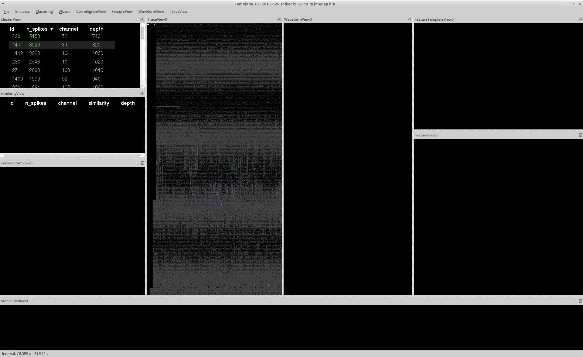
In the image above, you can see how these panels are arranged along with the type of plots that are generated. These panels can be rearranged depending on your personal preference. Further information on each view can be found by following these links:
- TraceView
- ClusterView
- SimilarityView
- CorrelogramView
- AmplitudeView
- WaveformView
- FeatureView
- FeatureTemplateView
There is also a detailed user guide for manual clustering
TraceView
The raw traces are plotted in TraceView automatically when the application launches. Detected events are highlighted in colour, each colour corresponds to a different cluster. If you select a cluster in Clusterview, events from this cluster are highlighted as is shown below:
The scaling of the traces can be adjusted using the drop down toolbar for TraceView, using the mouse (right click + drag) or keyboard shortcuts. TraceView shows only a subset of the total trace at any given time. The length of visible trace can be adjusted by using the command 'Widen Trace' (Ctrl + Alt + right) in the drop down menu.
The displayed interval is visible at the bottom of the GUI if you hover the mouse over TraceView.
You can also go directly to a specific time by selecting Go to from the TraceView menu.
NOTE: If the window of displayed traces is increased too much the template-gui's performance will decrease. It is therefore advisable to keep the window small and to shift the window using
Alt + left/right, rather than to increase the size of the visible trace.
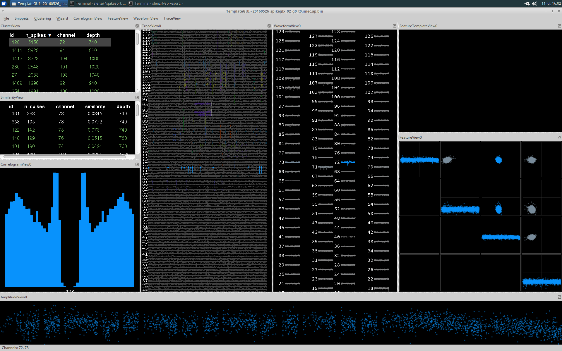
ClusterView and SimilarityView
ClusterView and SimilarityView both display a list of all the detected clusters, providing information regarding the cluster id, number of spikes (n_spikes), the channel with the largest amplitude events, and the corresponding depth of that channel. This list can be sorted according to any of these displayed parameters by clicking its name.
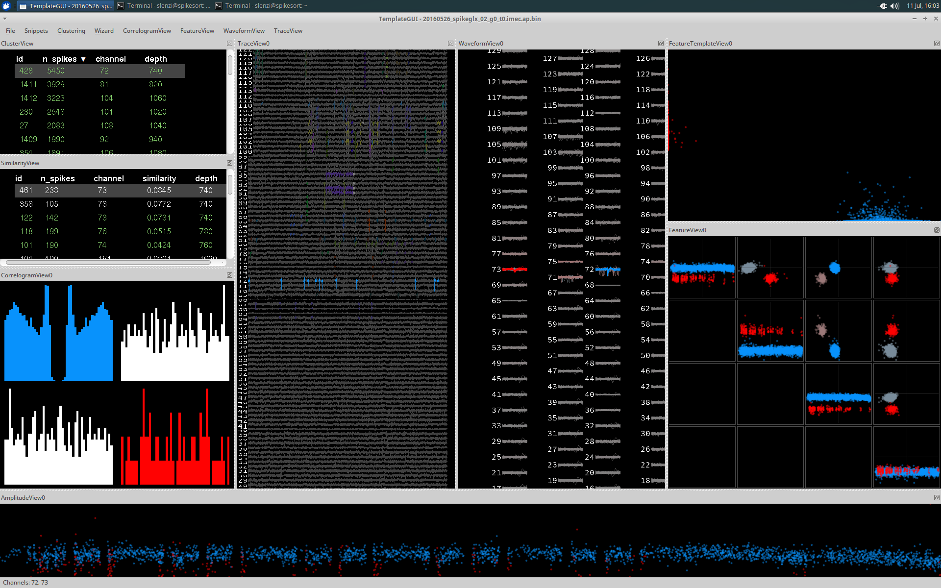
A cluster can be selected by clicking it (de-select with Ctrl and click), which results in plotting in all the other Views in blue (if selected from ClusterView) and red (if selected from the SimilarityView). Events from the cluster will also be highlighted in TraceView in the corresponding colours.
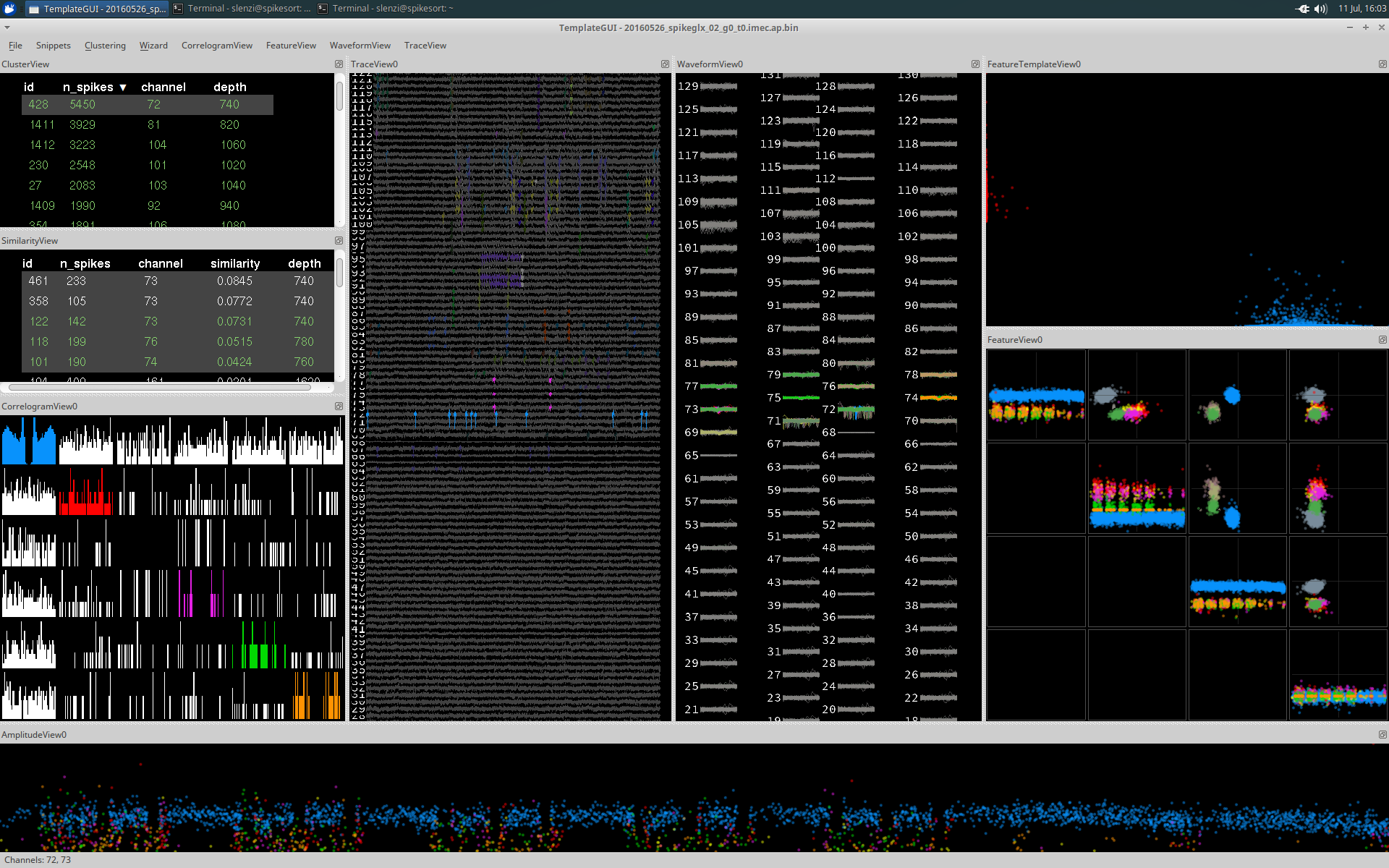
Additional clusters can be selected by holding Ctrl and selecting additional clusters. Shift + clicking will allow you to select a range. Each additional cluster is plotted in a different colour.
CorrelogramView
CorrelogramView displays the auto-correlograms of each cluster's spike trains in color (on the diagonal) and the cross-correlograms of each pair of spike trains from the selected clusters in white (on the off-diagonal).
By default the correlogram will show a window of 50ms and use a bin size of 1ms. These can both be adjusted using the CorrelogramView dropdown menu.
WaveformView
WaveformView plots a subset of the events of a cluster, displayed across all channels. Pressing the W key toggles between the individual traces and the average trace. If these are different between clusters it is very unlikely that they belong to the same cell. However, the converse is not true: similarity of waveforms is not sufficient in deciding if the two clusters arise from the same cell. If there are clearly two distinct groups of waveforms on the same channel, then it is possible that the cluster contains the events from several cells and should be considered for cluster splitting.
Not all waveforms are highlighted in the cluster colour. The colour intensity is an indication of the 'best channel' for detecting the given event. For well-isolated cells this is likely to be a subset of neighbouring channels. Some types of noise artefact may show up as having a very wide range of highlighted channels.
AmplitudeView
AmplitudeView displays the scaling of the template for each spike against time. This can indicate electrode drift, which would result in a consistent decrease or increase in amplitude/scaling with respect to time.
NOTE: Template scale factor is template-dependent so the points plotted are not necessarily comparable across templates.
FeatureTemplateView
FeatureView
FeatureView computes and displays principle component features for the best channel to aid the user in deciding whether events arise from the same or different clusters. The grid is arranged as follows:
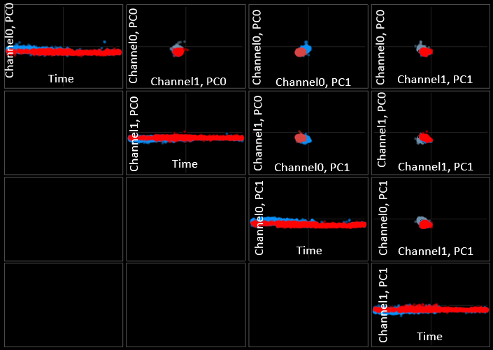
There are four features you can see (channel0 pc0 and 1, channel1 pc0 and 1). Each of these is has its own row and column to give you all combinations. The main diagonal is special, with time always on the x-axis.
Channel0 can be selected or changed using ctrl + left click on WaveformView, Channel1 can be selected or changed using ctrl + right click.
Additional user protocols
Merging: If you decide that multiple clusters are very likely to originate from the same cell, you should merge them into a single cluster by pressing the G key. This will merge all currently selected clusters. This will result in a new cluster_id and will remove the old ones.
Splitting: If the cluster has two clearly distinct groups of waveforms in the same channel then you should consider splitting the cluster into two groups. Try looking at the FeatureView. If you think the cluster may be made of two distinct groups encircle one of the groups by holding down Ctrl and left click around the group you would like to isolate. Each click creates a corner of a polygon selection. Once happy with the selection press K. Ideally this will successfully separate the two waveforms into two separate clusters. Ctrl + right click will undo your selection.
Assessing stability: stability can be inferred using the AmplitudeView and/or the first feature component that is displayed in the top left panel of the FeatureView. This component relates to the scaling of the templates, which should be fairly consistent over the whole recording time. If there is drift away from the neuron, then one would expect the waveforms to decrease.
Assessing refractory period: provided that n_spikes is large enough, and that events come from a single, well isolated cell, the ACG should be 0 at the centre of the x-axis corresponding to an extremely low or non existent correlation at lag 0). This is because of the refractory period of the neuron. If the cluster is made up of two distinct neurons, it is very likely that there will be no refractory period.
Keyboard shortcuts
Merging and splitting
Merge: G
Split: K
Select for splitting: Hold Ctrl and use the left mouse click (on FeatureView) to define each point of your desired polygon. Define a region around the events you want to separate and press K to split when you are satisfied with your selection. Ctrl + right mouse click will undo your selection.
Classifying clusters
Classify selected cluster(s) as 'good': Alt + G
Classify selected similar cluster(s) as 'good': Ctrl + G
Classify selected cluster(s) as 'MUA': Alt + M
Classify selected similar cluster(s) as 'MUA': Ctrl + M
Classify selected cluster(s) as 'noise': Alt + N
Classify selected similar cluster(s) as 'noise': Ctrl + N
Moving, zooming, adjusting
Drag: Left mouse button
Zoom: Right mouse button and drag
Increase scaling: Alt + up
Decrease scaling: Alt + down
Misc
Undo: Ctrl + Z
Select most similar/next most similar cluster: spacebar
"Snippets"
Snippets are commands you can enter quickly from the keyboard to perform certain actions. Start each snippet by typing a :. E.g. if you type exactly these characters:
:c 321[Enter]
Then cluster 321 will be selected.
* Available snippets:
* :c X Y Z - Select clusters X, Y, and Z
* :cb X - set correlogram bin size to X
* :cw X - set correlogram window width to X
All commands can be run as snippets. For example, :move, :merge, :recluster, and so on. The command name of every action is displayed in the status bar at the bottom of the window when you hover your mouse on any action in the menu bar.
A typical approach to manual clustering
Usage summary
1) If the waveforms are large with respect to the baseline (step 1) 2) there is a clear refractory period in the CCG (step 3) 3) potential merges and splits have been considered (steps 2-4) 4) then select 'move best to good' from the clustering drop down (or use the shortcut Alt + G). If you are unsure, or if any of these distinctions fail, then select 'move best to MUA', and if it is most likely noise 'move best to noise'. (step 5) 5) Once you are satisfied with your cluster classifications, select save from the ClusterView drop down menu. This will create a .csv file containing a list of cluster ids and their corresponding groups (good, MUA, noise). Saving will also make spike_clusters.npy, a file containing the cluster identities of each spike. These files are saved to the current directory (step 6).
Detailed guide
Step 1 - select a cluster from ClusterView
Is the amplitude very low?
Is the waveform shape noise-like?
Does the ACG reveal no evidence of a refractory period?
- If YES: label as MUA or noise, select next cluster
- If NO: select the most similar cluster to compare, move to next step.
Hint: hit the spacebar to rapidly select the most similar cluster
Step 2 - waveform similarity
Are the waveforms clearly distinct or do the clusters occupy a clearly different set of channels?
- If YES: these clusters are non-overlapping, select the next most similar cluster (hit the
spacebaragain) in SimilarityView and repeat step 2 - If NO (i.e. the waveforms are very similar): move to step 3
Step 3 - assess cross correlograms
In the ACG/CCGs, is there evidence that both neurons have good refractory periods, but the CCG shows no refractory period?
- Consider CorrelogramView. If the ACGs for each cluster are dissimilar and there is no refractory period visible in the CCG, they are not the same neuron; move on to next most similar (hit
Spacebaror select manuallyCtrl + click) - If the ACGs are similar and the CCG looks the same as both ACGs, then consider steps 4-6:
NOTE: if the number of events in a cluster is low, then the CCGs/ACGs are not reliable. If they are noisy, or have very few events per bin, then they do not tell the user much either way regarding potential merges and splits.
Step 4 consider FeatureView and AmplitudeView
4a - stability:
Do both neurons appear stable over time and/or they appear to drift into one another continuously? (see glossary: `stability`, and `amplitudes`)
4b - overlap in feature space:
Is there any evidence in the feature views that they form distinct clusters?
Are the clusters non-overlapping in all feature plots?
Do they occupy different areas in feature space?
- If 4a YES and 4b NO: the clusters should probably be merged (press the
Gkey to group them) - Otherwise select the next most similar cluster and start over from step 2
Step 5 - classify as good
Once all potential comparisons have been made, if there is a clear refractory period and there is no evidence that the cluster needs to be split, the cluster can be classified as 'good' (Alt + G). When a cluster is classified as 'good' it will appear in the Cluster and Similarity Views in green. If it is in any way unclear, then it should be classified as MUA. When a cluster is classified as 'MUA' (Alt + M) or 'noise' (Alt + N) it will appear in the Cluster and Similarity Views in light grey. There are additional packages for objective assessment of clustering quality.
Exceptions to this include bursting neurons, which are a special case. Action potential bursts usually consist of spikes/subclusters that differ in shape/amplitude. Waveforms and features may appear distinct, although the events belong to the same cluster. Clusters belonging to a burst from the same neuron have signature CCGs: the smaller of the two reliably follows the larger by a very short interval (1-3ms). This displays itself as a very clear asymmetric distribution, with a clear refractory period.
Step 6 - save your progress
The GUI keeps track of all decisions in a file called phy.log. The current classifications can be saved at any time with the command Ctrl + S.
Further advice
The decision-making process will vary slightly depending on the experimental question, and whether false positives or false negatives are more dangerous. Generally the aim is to produce as many well isolated neurons as possible (to a high level of confidence). As a rule of thumb uncertainty means excluding data.
For many applications, clusters with very few APs can be ignored (below 20). The error rate of Kilosort is very low (missed events ~1% ) and it is hard to know without good ACGs/CCGs to which cluster the events belong. The cutoff for this will vary between experiments.
Getting started with analysis
The primary files you will need for your analysis now are spike_times.npy and spike_clusters.npy, identifying the times and identities of every spike, along with cluster_group.tsv, which has the labels you gave to the clusters (noise/MUA/good).
If you are using Matlab, you will need the npy-matlab repository to load these data files. You can also make use of the spikes repository which has some functions you may find useful. Importantly, unlike Phy and Phy-contrib, spikes is provided "as-is" and is not guaranteed to work, nor to be stable, nor to be well-documented! But you may find parts useful, for example: * loadKSdir - load some of the useful pieces of information from the kilosort and manual sorting results into a struct * readClusterGroupsCSV - load the information from the cluster_group.tsv file with cluster labels * getWaveForms - extract some raw waveforms out of the original data file * templatesPositionsAmplitudes - compute some useful things about your spikes and their waveform shapes, like the position along the probe and the amplitudes * psthViewer - a simple GUI to quickly look at rasters and PSTHs aligned to some event, and scroll through your different clusters.
FAQ
-
I opened the GUI but don't have a waveform view or trace view. What happened?
- These views won't show if the data file isn't found or can't be loaded. So check that your params.py has the correct path for the data file and that it is the correct file.
-
How can I determine the waveform shape of cluster X now that I'm done with sorting?
- Phy does not save mean waveforms or waveform samples so you can't just load the answer. There are two ways to approach this.
- First, you can extract the raw waveforms at the spike times of cluster X and average them (e.g. in matlab use the getWaveForms function. More generally, memory-map the raw data file and simply read out the voltage data around the spikes times of interest).
- Second, you could just take the template shape for each cluster. If there were merges, then a single cluster will have spikes from multiple templates in it, and an approximation that may be good enough (depending on your purpose) is to just take the template that is associated with the greatest number of constituent spikes. E.g. just tally up how many times each template is in cluster 961 (maybe 1200 spikes from template 897 and 100 from template 654), take the max (897) and use that template. The peak channel, the waveform width, or the amplitude of template 897 will be a close approximation of the value for cluster 961 even though cluster 961 included spikes from template 897 as well as other templates (since only similar templates are merged). A function that computes the template for each cluster according to this logic can be found here.
Glossary
Definitions
Stability how consistent the recordings are over the recording period. For example, electrode drift during an experiment would be an example of instability.
Waveform amplitude is evaluated by looking at the waveforms. The decision of whether this is too low to be considered in the analysis is subjective.
Auto-correlogram (ACG): the pairwise cross correlations of...
Cross-correlogram (CCG): the cross correlogram of the ACGs
Multi-unit activity (MUA): category for cells that are not well isolated.
good: this classification is user determined, and is generally meant to be used to label cells that are well-isolated to a high level of confidence.
MUA: this is for clusters that fail to meet the good criteria, usually because they consist of poorly isolated cells (e.g. they do not have a clean refractory period).
noise: noisy waveforms are classified as noise (i.e. the waveform looks like an artefact or is present in an unrealistic/biologically unlikely set channels).
Similarity: is a variable in SimilarityView that indicates how similar a cluster is to the one selected in ClusterView. This should guide the user to clusters that should be considered for merging using the protocol in the user guide. High similarity does not necessarily mean the clusters should be merged. There is no hard cut off for considering similarity, but clusters with low similarity are very unlikely to need to be merged.